pg_stats: How Postgres Internal Stats Work
Introduction
I recently had the privilege of speaking at POSETTE 2026 about pg_stats and how Postgres internal statistics work (YouTube Recording). This post is a written companion to that talk – aimed at giving you a working understanding of what pg_stats is, how it’s populated, and how it shapes the decisions the query planner makes on your behalf.
Imagine a customers table that looks roughly like this:
CREATE TABLE customers (
    id          bigserial PRIMARY KEY,
    city        text NOT NULL,
    state       text NOT NULL,
    signup_date date NOT NULL
);
-- Insert 1,000,000 rows
Consider a query you’ve probably written many times:
SELECT * FROM customers WHERE state = 'CA';
With separate indexes on state and city, you might expect an index scan on state. But the EXPLAIN ANALYZE output may look something like this:
                              QUERY PLAN
-----------------------------------------------------------------
 Seq Scan on customers  (cost=0.00..19682.66 rows=173829 width=26)
                        (actual time=0.025..120.574 rows=172001 loops=1)
   Filter: (state = 'CA'::text)
   Rows Removed by Filter: 827972
   Buffers: shared hit=4601 read=2582
 Planning:   Buffers: shared hit=139
 Planning Time: 0.371 ms
 Execution Time: 128.136 ms
A sequential scan, even with an index available. We’ll get into the reasons for this today.
Query Plans Are Made by the Query Planner
When you submit a query to Postgres, the query planner is responsible for deciding how to execute it. You may assume the planner reads your actual data – it doesn’t. What it really reads is a summary of your data, stored in pg_statistic.
That summary tells the planner things like:
- How many distinct values appear in a column
- What the most common values are, and how often they show up
- What the rough distribution of values looks like across a range
- Whether the data is laid out on disk in roughly the same order as the column’s natural sort order
pg_statistic itself is a bit hard to read directly – the values are stored in formats optimized for the planner, not for humans. Fortunately, Postgres provides a view called pg_stats that exposes the same information in a far more readable form.
ANALYZE: How the Summary Gets Built
The summary in pg_statistic doesn’t populate itself. It’s built (and refreshed) by the ANALYZE command:
ANALYZE customers;
ANALYZE scans the table (or a sample of it), computes a handful of statistics per column, and writes the results into pg_statistic. Autovacuum runs ANALYZE for you in the background, but after large data loads or migrations, you’ll often want to run it manually.
Let’s look at what comes out of it. Using our customers table:
SELECT attname, n_distinct, null_frac, correlation
FROM pg_stats
WHERE tablename = 'customers'
ORDER BY attname;

   attname    | n_distinct | null_frac |  correlation
--------------+------------+-----------+--------------
 city         |      10106 |         0 |  0.0021338463
 id           |         -1 |         0 |             1
 signup_date  |       1822 |         0 |             1
 state        |         50 |         0 |    0.06440461
(4 rows)
A few things worth pointing out:
n_distinctis the estimated number of distinct values. Forstate, it’s exactly 50 – which lines up with the number of states in the United States.cityreports around 10,106, which is believable for U.S. cities. A value of-1in theidcolumn means the column is unique: every row has a distinct value.null_fracis the fraction of rows where the column isNULL. All four columns here areNOT NULL, so the values are all0.correlationis a number between-1and+1that estimates how well the on-disk physical ordering of the table matches the logical ordering of the column. A value of+1means the data is perfectly sorted on disk (e.g., an incrementingidcolumn or a date column in an append-only table). Values close to0mean the data is randomly ordered on disk relative to the column’s values. Values close to-1or+1encourage index scans; values near0discourage them. The docs go into more detail, but practically it acts as a penalty multiplier in the cost calculation.
Most Common Values (MCV)
ANALYZE also captures a list of the most common values in a column, along with their frequencies. These live in two parallel arrays: most_common_vals and most_common_freqs.
SELECT
    unnest(most_common_vals::text::text[]) AS state,
    unnest(most_common_freqs)              AS frequency
FROM pg_stats
WHERE tablename = 'customers' AND attname = 'state'
LIMIT 5;

 state |  frequency
-------+-------------
 CA    |  0.17403333
 TX    |      0.1165
 NY    |  0.08586667
 FL    |      0.0666
 IL    |      0.0474
(5 rows)
So CA appears in about 17.4% of the rows, TX in 11.6%, and so on. These frequencies feed directly into how the planner estimates rows – and therefore how it picks scan types.
Costs: How the Planner Picks a Plan
The planner makes its choices based on cost. Three of the more commonly-encountered cost parameters are:
random_page_cost– the cost of fetching a random page from disk (think: index scan plus heap fetch)seq_page_cost– the cost of fetching a page sequentially (sequential scan)cpu_tuple_cost– the cost of processing each row pulled out of a page
These costs, along with row estimates from pg_statistic, drive two big decisions:
Scan Type
- Sequential Scan
- Index Scan
- Bitmap Heap Scan
Join Type
- Nested Loop
- Hash Join
- Merge Join
The planner generates several candidate plans, calculates the cost of each, and picks the cheapest. Bad statistics lead to bad row estimates, which can lead to bad plan choice. As you can see, having good statistics is vital to query performance.
A Tale of Two States
Watch what happens when we query for CA versus WY:
EXPLAIN ANALYZE SELECT * FROM customers WHERE state = 'CA';
-- Seq Scan on customers  (cost=0.00..19682.66 rows=174029 ...)
--                        (actual time=0.042..50.257 rows=172001 loops=1)

EXPLAIN ANALYZE SELECT * FROM customers WHERE state = 'WY';
-- Index Scan using customers_state_idx on customers
--    (cost=0.42..13116.39 rows=4233 ...)
--    (actual time=0.045..21.238 rows=4300 loops=1)
CA matches about 18% of the table – around 180,000 rows. For every matching row, an index scan would need to look up the row in the index, fetch the page off disk, and pull the tuple out. Doing that 180,000 times turns out to be more expensive than just reading the whole table sequentially. So the planner picks a sequential scan.
WY, on the other hand, matches only about 4,000 rows. At that selectivity, the index scan wins by a wide margin.
We can confirm this is really about cost by forcing the issue. If we temporarily disable sequential scans, the planner is forced to use the index:
SET enable_seqscan = off;

EXPLAIN ANALYZE SELECT * FROM customers WHERE state = 'CA';
--  Index Scan using customers_state_idx on customers
--    (cost=0.42..32172.73 rows=170529 width=26)
--    (actual time=0.053..75.656 rows=172001 loops=1)
The planner’s original choice of a sequential scan (cost ~19,682) was cheaper than this forced index scan (cost ~32,172). The MCV statistics told the planner that CA shows up a lot, and the planner correctly judged that a sequential scan would be cheaper. Skewed data is exactly when MCV earns its keep.
Histograms: For Everything That Isn’t Equality
MCVs are great when you’re searching for specific values. But what about ranges – signup_date BETWEEN ..., or id > ...? For that, ANALYZE builds a histogram.
By default, the histogram has 100 buckets, each holding roughly the same number of rows (it’s an equi-depth histogram). You can look at the bucket boundaries:
SELECT (unnest(histogram_bounds::text::date[]))::date AS bucket_bound
FROM pg_stats
WHERE tablename = 'customers' AND attname = 'signup_date'
LIMIT 8;

 bucket_bound
--------------
 2018-01-01
 2018-03-01
 2018-04-28
 2018-07-04
 2018-09-05
 2018-10-28
 2018-12-27
 2019-02-14
(8 rows)
Each bucket here covers roughly two months – about 1% of the table. That’s fine for many cases, but if you have a large table with a skewed time distribution, you may want more precision.
Consider this side-by-side comparison:
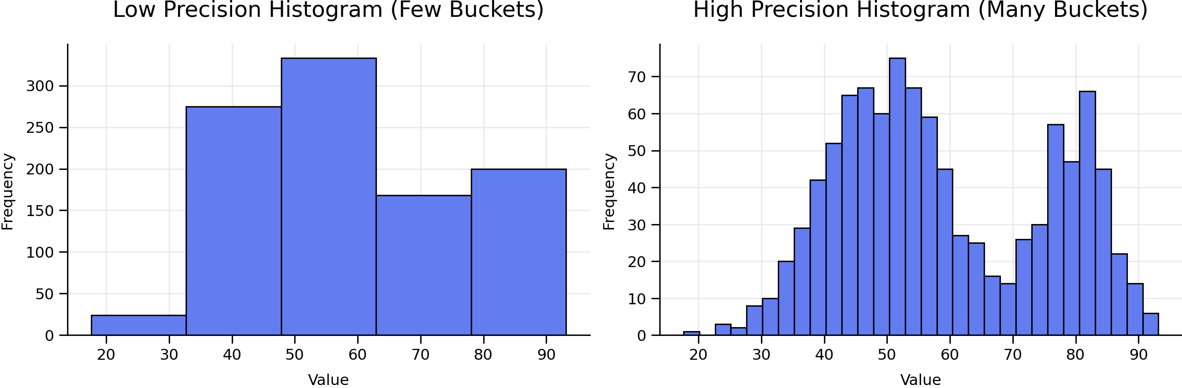
- A low-precision histogram (few buckets) might tell you “the most data lives somewhere between 30 and 65.”
- A high-precision histogram (many buckets) might tell you “the peak is between 50 and 52, with a clear dip around 65–70 and a second smaller peak near 80.”
Both are technically correct. Only one helps the planner make a good decision when your query is WHERE value BETWEEN 65 AND 70.
You can increase the bucket count on a per-column basis:
ALTER TABLE customers
    ALTER COLUMN signup_date SET STATISTICS 1000;
ANALYZE customers;
Now the same query shows buckets that are about two days wide instead of two months:
 bucket_bound
--------------
 2018-01-01
 2018-01-03
 2018-01-05
 2018-01-07
 2018-01-10
 2018-01-12
 2018-01-14
 2018-01-16
(8 rows)
Beware of trade-offs. More buckets means more precision, but also more work for ANALYZE and a larger pg_statistic row to traverse during planning. Don’t increase default_statistics_target across the entire database – target only the columns where you actually have problematic estimates.
Correlation Between Columns
So far we’ve looked at a single column at a time. Things get more interesting – and more wrong – when you filter on two columns at once:
EXPLAIN ANALYZE
SELECT * FROM customers
WHERE city = 'Cheyenne' AND state = 'WY';

-- Index Scan on customers  (cost=... rows=8 width=...)
--                          (actual rows=4012)
The planner estimates 8 rows, but the query returns 4,012. That’s a 500x miss.
This happens because, by default, the planner assumes columns are statistically independent:
\[P(\text{city} = \text{Cheyenne} \;\wedge\; \text{state} = \text{WY}) = P(\text{city}) \times P(\text{state})\]In reality, city and state are correlated. There’s basically one Cheyenne in the U.S., and it’s in Wyoming. (There’s also a Cheyenne, Oklahoma, but with a population of around 700, it doesn’t really move the needle.) So filtering on city = 'Cheyenne' is almost equivalent to filtering on state = 'WY', but the planner doesn’t know that.
Since Postgres 10, you can tell it:
CREATE STATISTICS customers_city_state (dependencies, ndistinct)
ON city, state FROM customers;

ANALYZE customers;
The dependencies and ndistinct arguments are statistic types – they tell Postgres what kind of cross-column information to track. After re-running ANALYZE:
EXPLAIN ANALYZE
SELECT * FROM customers
WHERE city = 'Cheyenne' AND state = 'WY';

-- Index Scan on customers  (cost=... rows=4087 width=...)
--                          (actual rows=4012)
The estimate of 4,087 versus actual 4,012 is essentially perfect. Just as importantly, this estimate now feeds correctly into any joins or aggregations that sit on top of this scan. Mis-estimates at the bottom of a plan tend to compound – a wrong scan choice deep in the tree can cause cascading mistakes in the joins above it. That’s part of why getting the foundational statistics right matters so much.
Note: Creating extended statistics isn’t free. It adds a small amount of overhead to
ANALYZEand to the query planning process itself. You should only create them when you’ve identified a clear case of mis-estimation due to correlated columns.
A Quick Checklist for Query Performance
When a query plan looks wrong, here’s roughly the order I work through:
- Compare estimated vs. actual rows. Run
EXPLAIN ANALYZEand look for the deepest node where the estimate disagrees with reality. That’s usually where the problem starts. - Check
pg_statsfor that column. Look atn_distinctand the MCV list. Do they match what you know about your data? - If the stats look stale, run
ANALYZE. This is especially common after a big batch load, a migration, or a partition swap. Autovacuum may not have caught up. - If estimates are still off on a single column, raise the statistics target.
ALTER TABLE ... ALTER COLUMN ... SET STATISTICS 1000;and re-ANALYZE. - If the bad estimate involves two columns in the same
WHEREclause, consider correlation. Create extended statistics on the pair. - Only after all of that should you consider rewriting the query – or reaching out for help.
Conclusion
The Postgres query planner is impressively good at its job, but it isn’t magic. It makes decisions based on a summary of your data, and the quality of those decisions is bounded by the quality of that summary. pg_stats is your window into what the planner thinks is true about your tables – and when reality and the planner’s beliefs diverge, that’s usually where bad plans come from.
The next time EXPLAIN ANALYZE surprises you, before you start setting enable_seqscan = off in production or rewriting the query out of frustration, take a look at pg_stats first. More often than not, the answer is there.
The Query Planner is only as smart as the statistics you feed it.